Marketing teams spend about 4 hours each day on manual, administrative, and operational tasks, according to HubSpot’s State of Marketing Report. The average marketer spends around 16 hours a week on routine tasks—nearly a third of their total work time on repetitive activities. According to WebFX marketing analytics research, 32% of sales representatives spend over an hour per day on manual data entry alone.
Google Sheets formulas can automate these repetitive calculations in seconds, transforming how marketers handle campaign data.
This guide provides over 56 formulas with specific marketing applications, teaching you how to transform raw numbers into actionable insights while reclaiming hours every week.
TL;DR
- Master 56+ formulas organized by marketing use case: campaign tracking, lead management, SEO reporting, time tracking, and ROI analysis
- Basic calculations (SUM, AVERAGE, COUNT) handle metrics aggregation while conditional logic (IF, AND, OR) creates automated performance flags.
- Lookup functions (VLOOKUP, INDEX/MATCH) merge data from multiple sources; INDEX/MATCH is more reliable than VLOOKUP for production dashboards.
- Text manipulation (CONCATENATE, SPLIT, REGEXEXTRACT) cleans keyword data and parses URLs for the SEO workflow.s
- Advanced automation combines QUERY and IMPORTRANGE for centralized reporting, and ARRAYFORMULA for bulk calculations.s
- Error handling with IFERROR and IFNA prevents dashboard failures; using absolute cell references ($A$1) ensures formulas remain functional when copied.
- Performance optimization matters: use closed ranges instead of entire columns, minimize volatile functions, and leverage named ranges for large datasets.s
- Real-time dashboards update automatically using IMPORTRANGE, QUERY, and conditional formatting, eliminating the need for manual reporting work.
- Know when to upgrade: Move to Looker Studio for visualization, BigQuery for massive datasets, or marketing automation tools when sheets slow down.

What Are Google Sheets Formulas (and Why They Matter for Marketing Data)
![]()
A formula is an instruction that begins with an equal sign (=) and tells Google Sheets to perform calculations or manipulate data across one or more cells. The basic formula syntax follows this structure:
=FUNCTION(argument1, argument2, …)
For marketers handling campaign data from multiple cells, formulas eliminate tedious manual work. Instead of copying metrics across spreadsheets or recalculating ROI every Monday morning, formulas process numerical and logical values instantly and update automatically when source data changes.
Core benefits for marketing teams:
- Automate repetitive calculations across cell ranges
- Reduce human errors in performance dashboards
- Create shareable, collaborative data tools that update in real-time
- Build custom KPIs using complex formulas tailored to your metrics
- Enable fast decision-making with live data analysis
Think of formulas as your personal data analyst—working 24/7 without coffee breaks.
How to Use Formulas in Google Sheets (Quick Start)
Never written a formula before? Here’s the five-step process to create formulas in any empty cell:
- Click the specified cell where you want the results
- Type = (the equal sign signals you’re creating a formula)
- Enter a function name like SUM or AVERAGE
- Select your cell range or type the cell address manually
- Close with ) and press Enter
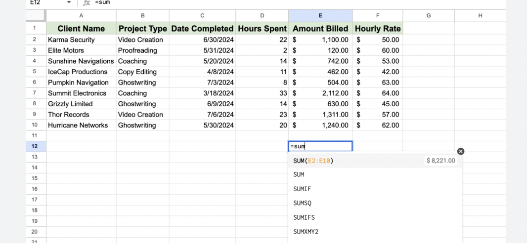
Example: To sum values in cells A2 through A10:
=SUM(A2:A10)
Fill handle trick: Drag the small square at the bottom-right corner of any cell to copy the same formula down multiple rows or across multiple columns. Google Sheets automatically adjusts relative references.
Pro move—Combining formulas: Chain multiple calculations together:
=SUM(A2:A10)*AVERAGE(B2:B10)
This multiplies total clicks by average cost-per-click—giving you instant campaign spend calculations without creating helper columns.
The Most Essential Google Sheets Formulas for Marketers

Campaign Tracking & Analytics
1. SUM() – Total Your Metrics
Adds all the values in a specified range.
Formula syntax:
=SUM(range)
Marketing example:
=SUM(B2:B50)
Totals ad spend across 49 campaigns. Use this for monthly budget tracking, total impressions, or aggregate clicks.
2. AVERAGE() – Calculate Mean Performance
Returns the average of numerical values in a cell range.
Formula syntax:
=AVERAGE(range)
Marketing example:
=AVERAGE(C2:C50)
Finds average conversion rate across campaigns. Essential for benchmark comparisons.
3. COUNT() – Count Numeric Entries
Counts how many entries contain numerical values.
Formula syntax:
=COUNT(range)
Marketing example:
=COUNT(D2:D50)
Counts campaigns with recorded conversions (ignores empty cells).
4. COUNTA() – Count Non-Empty Cells
Counts all non-empty cells regardless of data type.
Formula syntax:
=COUNTA(range)
Marketing example:
=COUNTA(E2:E50)
Counts active campaign names to track how many campaigns are running.
5. IF() – Create Conditional Logic
Returns one value if a logical expression is true, another if false.
Formula syntax:
=IF(logical_test, value_if_true, value_if_false)
Marketing example:
=IF(D2>1.5, “High ROI”, “Needs Optimization”)
Automatically labels campaigns based on performance. No manual highlighting needed.
6. AND() – Test Multiple Conditions
Returns TRUE only if all conditions are met.
Formula syntax:
=AND(logical_expression1, logical_expression2, …)
Marketing example:
=IF(AND(B2>1000, C2<2), “Winning Campaign”, “Review”)
Flags campaigns with 1000+ conversions AND under $2 CPA.
7. OR() – Test Any Condition
Returns TRUE if any condition is met.
Formula syntax:
=OR(logical_expression1, logical_expression2, …)
Marketing example:
=IF(OR(D2>5, E2<0.5), “Action Required”, “Monitor”)
Alerts when either CPA is too high OR CTR is too low.
8. ROUND() – Clean Decimal Places
Rounds a number to a specified number of decimal places.
Formula syntax:
=ROUND(value, num_digits)
Marketing example:
=ROUND(A2, 2)
Converts 3.456789 to 3.46 for cleaner reports.
9. TEXT() – Format Numbers as Text
Converts numerical values to text with specified formatting.
Formula syntax:
=TEXT(value, format)
Marketing example:
=TEXT(B2, “$#,##0.00”)
Displays ad spend as “$1,234.56” instead of raw numbers.
10. SUMPRODUCT() – Multiply Then Sum
Multiplies corresponding values in arrays and returns the sum.
Formula syntax:
=SUMPRODUCT(array1, array2, …)
Marketing example:
=SUMPRODUCT(B2:B50, C2:C50)
Multiplies clicks by cost-per-click for each campaign, then totals—instant total ad spend across all campaigns.
Lead & Customer Data Management
11. VLOOKUP() – Vertical Lookup
Searches the first column of a range and returns a corresponding value from a specified column.
Formula syntax:
=VLOOKUP(search_key, range, index, [is_sorted])
Marketing example:
=VLOOKUP(A2, LeadSheet!A:C, 3, FALSE)
Finds lead email in column A, searches LeadSheet, returns lead score from the third column. Essential for merging CRM data with campaign results.
Important: Set is_sorted to FALSE for exact matches. TRUE only works with sorted data.
12. HLOOKUP() – Horizontal Lookup
Like VLOOKUP but searches rows instead of columns.
Formula syntax:
=HLOOKUP(search_key, range, index, [is_sorted])
Marketing example:
=HLOOKUP(“Q1”, A1:E10, 5, FALSE)
Finds “Q1” in the first row, returns the corresponding value from the fifth row down.
13. INDEX() – Return Value by Position
Returns the value of a cell at a specified row and column within a range.
Formula syntax:
=INDEX(range, row, [column])
Marketing example:
=INDEX(B2:B100, 10)
Returns the 10th value in column B—useful for referencing specific positions.
14. MATCH() – Find Relative Position
Returns the relative position of a value within a range.
Formula syntax:
=MATCH(search_key, range, [search_type])
Marketing example:
=MATCH(“Facebook”, A2:A100, 0)
Finds which row number contains “Facebook” in your campaign list.
15. INDEX/MATCH Combination – Superior Lookup
Combines INDEX and MATCH for flexible lookups that won’t break.
Formula syntax:
=INDEX(return_range, MATCH(lookup_value, lookup_range, 0))
Marketing example:
=INDEX(C2:C100, MATCH(E2, A2:A100, 0))
Searches for campaign name in E2, finds its position in column A, returns the corresponding value from column C (like conversion rate). Unlike VLOOKUP, this works even if columns are rearranged.
16. IMPORTRANGE() – Link Multiple Spreadsheets
Imports a cell range from another Google Sheets document.
Formula syntax:
=IMPORTRANGE(“spreadsheet_url”, “range_string”)
Marketing example:
=IMPORTRANGE(“https://docs.google.com/spreadsheets/d/abc123”, “Facebook Ads!A1:D50″)
Pulls Facebook ad data from one spreadsheet into your master dashboard. You’ll need to grant access permission the first time.
17. QUERY() – SQL-Style Data Manipulation
Runs a Google Visualization API query across data.
Formula syntax:
=QUERY(range, query_string, [headers])
Marketing example:
=QUERY(A1:F100, “SELECT A, SUM(D) WHERE B=’Facebook’ GROUP BY A ORDER BY SUM(D) DESC”)
Aggregates total conversions by campaign name for Facebook campaigns only, sorted highest to lowest. This single formula replaces multiple pivot tables.
18. ARRAYFORMULA() – Apply Formulas to Entire Ranges
Enables array calculations across one or more ranges without dragging.
Formula syntax:
=ARRAYFORMULA(array_formula)
Marketing example:
=ARRAYFORMULA(B2:B*C2:C)
Multiplies every value in column B by its corresponding value in column C instantly—no fill handle needed. Updates automatically when you add new rows.
19. UNIQUE() – Remove Duplicates
Returns only unique values from a range.
Formula syntax:
=UNIQUE(range)
Marketing example:
=UNIQUE(A2:A500)
Extracts unique campaign names from a list with duplicate entries.
20. SORT() – Order Data Automatically
Sorts rows of a range based on specified column(s).
Formula syntax:
=SORT(range, sort_column, is_ascending, [sort_column2, …])
Marketing example:
=SORT(A2:D100, 4, FALSE)
Sorts campaigns by conversion rate (column 4) in descending order—highest performers first.
SEO, Content & Keyword Reporting
21. CONCATENATE() – Join Text Strings
Combines text from multiple cells into a single cell.
Formula syntax:
=CONCATENATE(string1, string2, …)
Marketing example:
=CONCATENATE(A2, “ – “, B2, “ | “, C2)
Combines “Best Coffee Makers”, “2025 Guide”, and “Reviews” into “Best Coffee Makers – 2025 Guide | Reviews” for meta titles.
22. JOIN() – Concatenate with Delimiter
Joins text from a range using a specified delimiter.
Formula syntax:
=JOIN(delimiter, value_or_array1, [value_or_array2, …])
Marketing example:
=JOIN(“, “, A2:A5)
Combines multiple keywords into a comma-separated list: “keyword1, keyword2, keyword3, keyword4”
23. SUBSTITUTE() – Replace Text
Replaces existing text with new text.
Formula syntax:
=SUBSTITUTE(text, old_text, new_text, [occurrence])
Marketing example:
=SUBSTITUTE(A2, “http://”, “https://”)
Updates old URLs to secure protocol—essential for technical SEO audits.
24. LOWER() – Convert to Lowercase
Converts text to all lowercase letters.
Formula syntax:
=LOWER(text)
Marketing example:
=LOWER(A2)
Standardizes keyword data: “Best COFFEE makers” becomes “best coffee makers”
25. UPPER() – Convert to Uppercase
Converts text to all uppercase letters.
Formula syntax:
=UPPER(text)
Marketing example:
=UPPER(A2)
Useful for creating UTM parameters that require capitalization.
26. PROPER() – Title Case Conversion
Capitalizes the first letter of each word.
Formula syntax:
=PROPER(text)
Marketing example:
=PROPER(A2)
Transforms “best coffee makers” to “Best Coffee Makers” for headers.
27. SPLIT() – Divide Text by Delimiter
Divides text around a specified character and places each fragment in a separate cell.
Formula syntax:
=SPLIT(text, delimiter)
Marketing example:
=SPLIT(A2, “/”)
Breaks “example.com/blog/post-title” into three cells: “example.com”, “blog”, “post-title”
28. LEFT() – Extract Left Characters
Returns a specified number of characters from the start of text.
Formula syntax:
=LEFT(text, num_chars)
Marketing example:
=LEFT(A2, 5)
Extracts first 5 characters—useful for category codes in campaign names.
29. RIGHT() – Extract Right Characters
Returns a specified number of characters from the end of text.
Formula syntax:
=RIGHT(text, num_chars)
Marketing example:
=RIGHT(A2, 4)
Extracts year from dates formatted as “Campaign_Name_2025”
30. MID() – Extract Middle Characters
Returns characters from the middle of text.
Formula syntax:
=MID(text, starting_at, num_chars)
Marketing example:
=MID(A2, 8, 10)
Extracts 10 characters starting at position 8—perfect for parsing structured campaign codes.
31. FIND() – Locate Text Position
Returns the position of a text string within another string.
Formula syntax:
=FIND(search_for, text_to_search, [starting_at])
Marketing example:
=MID(A2, FIND(“utm_source=”, A2)+11, 10)
Finds where “utm_source=” appears in a URL, then extracts the next 10 characters—isolating the traffic source.
32. TRIM() – Remove Extra Spaces
Removes leading, trailing, and repeated spaces.
Formula syntax:
=TRIM(text)
Marketing example:
=TRIM(A2)
Cleans imported data: ” keyword phrase ” becomes “keyword phrase”
33. LEN() – Count Characters
Returns the length of text.
Formula syntax:
=LEN(text)
Marketing example:
=LEN(A2)
Checks if meta descriptions exceed 160 characters.
34. FILTER() – Show Only Matching Rows
Returns only rows that meet specified criteria.
Formula syntax:
=FILTER(range, condition1, [condition2, …])
Marketing example:
=FILTER(A2:D100, B2:B100>1000, C2:C100<5)
Shows only blog posts with 1000+ monthly visits AND under 5% bounce rate.
35. REGEXMATCH() – Test for Pattern
Tests if text matches a regular expression pattern.
Formula syntax:
=REGEXMATCH(text, regular_expression)
Marketing example:
=REGEXMATCH(A2, “utm_source=”)
Returns TRUE if cell contains a UTM source parameter—great for validating tracking links.
36. REGEXEXTRACT() – Extract Pattern Match
Extracts text matching a regular expression.
Formula syntax:
=REGEXEXTRACT(text, regular_expression)
Marketing example:
=REGEXEXTRACT(A2, “utm_source=([^&]+)”)
Pulls the utm_source value from a URL: extracts “facebook” from “…utm_source=facebook&utm_medium=…”
Marketing Calendar & Time Tracking
37. TODAY() – Current Date
Returns the current date (updates daily).
Formula syntax:
=TODAY()
Marketing example:
=B2-TODAY()
Shows days remaining until campaign end date—creates self-updating countdown.
38. NOW() – Current Date and Time
Returns the current date and time (updates continuously).
Formula syntax:
=NOW()
Marketing example:
=NOW()
Timestamps when data was last refreshed.
39. DATE() – Construct Date from Parts
Creates a date from year, month, and day values.
Formula syntax:
=DATE(year, month, day)
Marketing example:
=DATE(2025, 3, 15)
Creates March 15, 2025—useful when building campaign calendars from separate columns.
40. DATEDIF() – Calculate Date Differences
Calculates the difference between two dates.
Formula syntax:
=DATEDIF(start_date, end_date, unit)
Marketing example:
=DATEDIF(A2, B2, “D”)
Returns campaign length in days. Use “M” for months, “Y” for years.
41. EOMONTH() – End of Month
Returns the last day of a month.
Formula syntax:
=EOMONTH(start_date, months)
Marketing example:
=EOMONTH(A2, 0)
Finds the last day of the month for any date—perfect for monthly report deadlines.
42. NETWORKDAYS() – Count Workdays
Calculates working days between two dates.
Formula syntax:
=NETWORKDAYS(start_date, end_date, [holidays])
Marketing example:
=NETWORKDAYS(A2, B2)
Counts business days in a campaign period (excludes weekends automatically).
43. WORKDAY() – Add Business Days
Returns a date after a specified number of working days.
Formula syntax:
=WORKDAY(start_date, num_days, [holidays])
Marketing example:
=WORKDAY(A2, 10)
Calculates delivery date 10 business days from order—useful for project timelines.
44. YEARFRAC() – Fraction of Year
Calculates the fraction of a year between two dates.
Formula syntax:
=YEARFRAC(start_date, end_date, [basis])
Marketing example:
=YEARFRAC(A2, B2)
Useful for prorating annual budgets: multiply annual budget by this fraction for partial-year campaigns.
Ad & ROI Analysis
45. SUMIF() – Conditional Sum
Sums cells that meet a specific criteria.
Formula syntax:
=SUMIF(range, criterion, [sum_range])
Marketing example:
=SUMIF(B2:B50, “Facebook”, C2:C50)
Totals ad spend (column C) only for Facebook campaigns (column B).
46. COUNTIF() – Conditional Count
Counts cells that meet a criterion.
Formula syntax:
=COUNTIF(range, criterion)
Marketing example:
=COUNTIF(D2:D50, “>100”)
Counts how many campaigns generated more than 100 conversions.
47. AVERAGEIF() – Conditional Average
Averages cells that meet a criterion.
Formula syntax:
=AVERAGEIF(range, criterion, [average_range])
Marketing example:
=AVERAGEIF(B2:B50, “Google”, C2:C50)
Calculates average CPC for Google Ads campaigns only.
48. SUMIFS() – Multiple Criteria Sum
Sums cells that meet multiple criteria.
Formula syntax:
=SUMIFS(sum_range, criteria_range1, criterion1, [criteria_range2, criterion2, …])
Marketing example:
=SUMIFS(D2:D50, B2:B50, “Facebook”, C2:C50, “>1000”)
Sums conversions from Facebook campaigns with 1000+ impressions.
49. COUNTIFS() – Multiple Criteria Count
Counts cells meeting multiple criteria.
Formula syntax:
=COUNTIFS(criteria_range1, criterion1, [criteria_range2, criterion2, …])
Marketing example:
=COUNTIFS(B2:B50, “Email”, D2:D50, “>2”)
Counts email campaigns with ROI above 2.
50. AVERAGEIFS() – Multiple Criteria Average
Averages cells meeting multiple criteria.
Formula syntax:
=AVERAGEIFS(average_range, criteria_range1, criterion1, [criteria_range2, criterion2, …])
Marketing example:
=AVERAGEIFS(E2:E50, B2:B50, “Instagram”, D2:D50, “>50”)
Average engagement rate for Instagram campaigns with 50+ conversions.
51. IFERROR() – Handle Errors Gracefully
Returns a specified value if a formula results in an error.
Formula syntax:
=IFERROR(value, value_if_error)
Marketing example:
=IFERROR(C2/D2, 0)
If the division operation fails (dividing by an empty cell), displays 0 instead of #DIV/0!
52. IFNA() – Handle N/A Errors
Returns a specified value if a formula results in #N/A.
Formula syntax:
=IFNA(value, value_if_na)
Marketing example:
=IFNA(VLOOKUP(A2, Data!A:B, 2, FALSE), “No Match”)
Shows “No Match” when VLOOKUP can’t find a value instead of error messages.
53. MIN() – Find Minimum Value
Returns the minimum value from a range.
Formula syntax:
=MIN(value1, [value2, …])
Marketing example:
=MIN(C2:C50)
Identifies your lowest-cost campaign—useful for finding efficiency benchmarks.
54. MAX() – Find Maximum Value
Returns the maximum value from a range.
Formula syntax:
=MAX(value1, [value2, …])
Marketing example:
=MAX(D2:D50)
Finds your highest-converting campaign for replication strategies.
55. MEDIAN() – Find Middle Value
Returns the median (middle) value from a range.
Formula syntax:
=MEDIAN(value1, [value2, …])
Marketing example:
=MEDIAN(B2:B50)
Finds median CTR—more accurate than average when you have outliers.
56. MODE() – Find Most Common Value
Returns the most frequently occurring value.
Formula syntax:
=MODE(value1, [value2, …])
Marketing example:
=MODE(C2:C50)
Identifies the most common conversion count—helps spot typical performance.
Advanced Formula Combinations for Automation
INDEX + MATCH: The VLOOKUP Replacement
Why it’s better: VLOOKUP breaks when you insert columns and only searches right. INDEX/MATCH is flexible and resilient.
Formula:
=INDEX(C2:C100, MATCH(1, (A2:A100=E2)*(B2:B100=F2), 0))
This performs a two-way lookup—finds rows matching both platform (column A) AND date (column B), then returns data from column C. Use Ctrl+Shift+Enter for array formulas.
IF + ISBLANK: Bulletproof Dashboards
The problem: Formulas fail when referenced cells are empty.
The solution:
=IF(ISBLANK(A2), “Pending”, IF(B2>1000, “Success”, “Monitor”))
Only performs calculations when data exists. Shows “Pending” for incomplete rows instead of breaking.
QUERY + IMPORTRANGE: Centralized Multi-Sheet Reporting
Pull and analyze data from multiple spreadsheets:
=QUERY(IMPORTRANGE(“spreadsheet_url”, “Sheet1!A:F”), “SELECT Col1, SUM(Col4), AVG(Col5) WHERE Col2=’Q1′ GROUP BY Col1 ORDER BY SUM(Col4) DESC”)
This single formula:
- Imports data from another spreadsheet
- Filters to Q1 only
- Aggregates conversions by campaign
- Calculates average CPC
- Sorts by performance
Updates automatically when source data changes—perfect for client dashboards.
ARRAYFORMULA + REGEXEXTRACT: Bulk URL Parsing
Extract UTM parameters from entire columns at once:
=ARRAYFORMULA(IF(A2:A<>””, REGEXEXTRACT(A2:A, “utm_source=([^&]+)”), “”))
Processes hundreds of URLs instantly—no dragging formulas. The IF check prevents errors on empty cells.
SUMPRODUCT + Multiple Conditions: Advanced Aggregation
Calculate weighted metrics without helper columns:
=SUMPRODUCT((A2:A50=”Facebook”)*(B2:B50>100)*(C2:C50)*(D2:D50))
This multiplies clicks (C) by conversion rate (D) but only for Facebook campaigns with 100+ impressions. All in one formula.
Nested IF + AND/OR: Complex Campaign Logic
Multi-tier campaign classification:
=IF(AND(B2>5000, C2>0.05), “Tier 1″, IF(AND(B2>1000, C2>0.03), “Tier 2″, IF(B2>500, “Tier 3″, “Low Priority”)))
Classifies campaigns into four tiers based on spend and conversion rate.
Common Mistakes (and How to Fix Them)
Mistake #1: Misusing VLOOKUP with Unsorted Data
Problem: Setting the fourth parameter to TRUE when data isn’t sorted causes wrong matches.
Fix: Always use FALSE for exact matches:
=VLOOKUP(A2, Data!A:C, 2, FALSE)
Or switch to INDEX/MATCH which doesn’t have this limitation.
Mistake #2: Forgetting Absolute vs Relative Cell References
When copying formulas, references shift automatically—sometimes that’s wrong.
| Reference Type | Example | Behavior When Copied |
| Relative | A1 | Shifts (A1 becomes B2 when copied right and down) |
| Absolute | $A$1 | Stays fixed |
| Mixed Column | $A1 | Column fixed, row shifts |
| Mixed Row | A$1 | Row fixed, column shifts |
When to use absolute: Locking cell references to a single conversion rate or budget figure used across multiple calculations.
Example:
=B2*$E$1
Multiplies varying clicks (B2) by a fixed CPC stored in E1. When copied down, clicks update but CPC stays constant.
Mistake #3: Performance Issues with Large Datasets
Symptoms: Sheets takes 30+ seconds to recalculate, or you see “Loading…” frequently.
Solutions:
Use Named Ranges instead of long cell addresses:
- Select your data range
- Data → Named ranges → Create
- Reference as =SUM(MonthlyBudget) instead of =SUM(A2:A1000)
Replace nested IFs with VLOOKUP/INDEX/MATCH:
❌ Slow:
=IF(A2=”Facebook”,10,IF(A2=”Google”,15,IF(A2=”LinkedIn”,20,IF(A2=”Twitter”,8,5))))
✅ Fast:
=VLOOKUP(A2, Rates!A:B, 2, FALSE)
Turn off automatic calculation for massive sheets:
- File → Settings → Calculation
- Choose “On change and every minute” or “On change”
Mistake #4: Not Handling Errors in Formula Chains
One error breaks everything downstream.
Problem formula:
=C2/D2
When D2 is empty, you get #DIV/0! and every formula referencing this cell fails.
Protected formula:
=IFERROR(C2/D2, 0)
Now empty cells return 0, and your dashboard keeps working.
Understanding Error Messages
| Error Code | What It Means | Common Causes | How to Fix |
| #REF! | Invalid cell reference | Deleted a referenced cell | Update the cell address in your formula |
| #VALUE! | Wrong data type | Text in a math formula | Check that numerical values are formatted as numbers, not text |
| #N/A | Value not available | VLOOKUP can’t find match | Verify lookup value exists; use IFNA() to handle gracefully |
| #DIV/0! | Division by zero | Dividing by empty cell or zero | Wrap in IFERROR() or check for zero first |
| #NAME? | Unrecognized function | Misspelled function name | Check spelling; verify function exists |
| #NUM! | Invalid numeric value | Calculation produces impossible number | Check your math logic |
| #ERROR! | Generic error | Various causes | Check formula syntax carefully |
Beyond Basics: Using Google Sheets Like a Marketing Pro
SPARKLINE(): Dashboard Visualizations in Cells
Create miniature charts contained within a single cell.
Formula syntax:
=SPARKLINE(data, [options])
Line chart example:
=SPARKLINE(B2:B30, {“charttype”, “line”; “color”, “blue”; “linewidth”, 2})
Column chart for weekly performance:
=SPARKLINE(C2:C8, {“charttype”, “column”; “color”, “green”})
Win/loss indicator:
=SPARKLINE(D2:D12, {“charttype”, “winloss”; “color”, “green”; “negcolor”, “red”})
Shows green bars for gains, red for losses—perfect for quick performance scanning.
Building Self-Updating Dashboards
Three-formula power combination:
- Import data from multiple sources:
=IMPORTRANGE(“Facebook_Ads_URL”, “Data!A:F”)
=IMPORTRANGE(“Google_Ads_URL”, “Data!A:F”)
- Combine and filter:
=QUERY({IMPORTRANGE(“URL1″,”Data!A:F”);IMPORTRANGE(“URL2″,”Data!A:F”)}, “SELECT Col1, SUM(Col4), AVG(Col5) WHERE Col2 CONTAINS ‘Active’ GROUP BY Col1 ORDER BY SUM(Col4) DESC”)
- Add conditional formatting (Format → Conditional formatting) based on performance thresholds.
This creates a live dashboard that updates whenever team members edit source spreadsheets—no manual refreshing needed.
RANDBETWEEN() – Generate Test Data
Create sample data for testing formulas.
Formula syntax:
=RANDBETWEEN(bottom, top)
Marketing example:
=RANDBETWEEN(100, 10000)
Generates a uniformly random integer between 100 and 10,000—useful for creating mock campaign data when building templates.
TRANSPOSE() – Flip Rows to Columns
Converts vertical data to horizontal (or vice versa).
Formula syntax:
=TRANSPOSE(array_or_range)
Marketing example:
=TRANSPOSE(A1:A12)
Converts 12 monthly rows into columns for horizontal comparison charts.
HYPERLINK() – Create Clickable Links
Turns URLs into clickable text.
Formula syntax:
=HYPERLINK(url, [link_label])
Marketing example:
=HYPERLINK(“https://analytics.google.com/report/”&A2, “View Campaign”)
Creates clickable “View Campaign” links that include campaign IDs from column A.
GOOGLETRANSLATE() – Translate Text
Automatically translates text between languages.
Formula syntax:
=GOOGLETRANSLATE(text, [source_language], [target_language])
Marketing example:
=GOOGLETRANSLATE(A2, “en”, “es”)
Translates English ad copy to Spanish for international campaigns.
COUNTUNIQUE() – Count Distinct Values
Returns how many unique values exist in a range.
Formula syntax:
=COUNTUNIQUE(value1, [value2, …])
Marketing example:
=COUNTUNIQUE(A2:A500)
Counts how many different channels you’re running campaigns across—ignores duplicates.
Advanced Data Validation with Formulas
Create dynamic dropdown lists that change based on other selections.
Setup:
- Create a named range for your source data
- Data → Data validation → Criteria: “List from a range”
- Use INDIRECT() for dependent dropdowns:
=INDIRECT(B2&”_List”)
When someone selects “Facebook” in B2, the dropdown shows options from a named range called “Facebook_List”.
Custom Functions with Apps Script
When built-in formulas aren’t enough, create your own.
Example: Get campaign data from APIs
function getAdSpend(campaignID) {
// Your API call here
var response = UrlFetchApp.fetch(apiURL + campaignID);
var data = JSON.parse(response);
return data.spend;
}
Use in sheets as: =getAdSpend(A2)
Performance Optimization Techniques
Use Closed Ranges Instead of Open Columns
❌ Slow (scans entire column):
=SUMIF(A:A, “Facebook”, B:B)
✅ Fast (scans only specified cells):
=SUMIF(A2:A500, “Facebook”, B2:B500)
Replace Volatile Functions When Possible
These recalculate constantly and slow down sheets:
- NOW()
- TODAY()
- RAND()
- RANDBETWEEN()
- INDIRECT()
Strategy: If you need a timestamp, enter it once manually or use a script instead of NOW() in every row.
Limit IMPORTRANGE Usage
Each IMPORTRANGE creates a persistent connection. Too many slow down your sheet.
Better approach: Import once to a data tab, then reference that tab throughout your sheet:
DataTab: =IMPORTRANGE(“URL”, “Sheet!A:F”)
Analysis: =QUERY(DataTab!A:F, “SELECT…”)
Use Filter Views Instead of FILTER() for Exploration
When you’re exploring data interactively, use Filter Views (Data → Create a filter view) instead of FILTER() formulas. They don’t recalculate constantly.
Save FILTER() for automated reports that need to update dynamically.
Minimize Array Formulas
Array formulas (ones requiring Ctrl+Shift+Enter) are powerful but slow with large datasets.
Alternative: Use ARRAYFORMULA() with proper logic instead:
=ARRAYFORMULA(IF(A2:A<>””, B2:B*C2:C, “”))
The IF(A2:A<>””,…) check prevents processing empty rows.
How to Learn Google Sheets Formulas Faster

Start with a Real Project
Don’t memorize syntax in isolation. Pick a report you create manually every week and automate it.
Beginner projects:
- Social media engagement tracker with weekly totals
- Email campaign ROI calculator
- Content calendar with automatic deadline reminders
Intermediate projects:
- Multi-channel ad spend dashboard
- Lead scoring system with conditional formatting
- SEO keyword tracker with rank change alerts
Advanced projects:
- Automated client reporting from multiple data sources
- Budget allocation optimizer with scenario modeling
- A/B test significance calculator
Follow These YouTube Creators
- Ben Collins – Advanced formula techniques and Google Sheets tips
- Better Sheets – Practical marketing and business templates
- ExcelIsFun – Comprehensive tutorials (Excel-focused but concepts apply)
- Leila Gharani – Data analysis and visualization techniques
- Sheets Help – Quick tips and formula explanations
Learn by Chaining Formulas
Master one formula, then combine it with another. This progression builds real understanding:
- Start: =SUM(B2:B10)
- Add logic: =IF(A2=”Facebook”, SUM(B2:B10), 0)
- Handle errors: =IFERROR(IF(A2=”Facebook”, SUM(B2:B10), 0), “No data”)
- Make it dynamic: =IFERROR(IF(A2=”Facebook”, SUMIF(C:C,”Active”,B:B), 0), “No data”)
Each step adds one new concept to master.
Keep a Personal Formula Library
Every time you solve a problem, document it in a dedicated “Formulas” sheet:
| Use Case | Formula | Notes |
| Calculate ROI | =(Revenue-Cost)/Cost | Returns decimal (0.50 = 50% ROI) |
| Days until deadline | =B2-TODAY() | Negative = overdue |
| Campaign status | =IF(C2<TODAY(),”Completed”,”Active”) | Based on end date |
Your own examples stick better than generic tutorials because they solve YOUR specific problems.
Use Google’s Built-In Formula Help
When typing a formula, Google Sheets shows:
- Function syntax
- Parameter descriptions
- Example usage
Press Ctrl + Shift + Enter in the formula bar to see full documentation.
Join Communities
Reddit:
- r/googlesheets – Active community answering questions daily
- r/sheets – Formula help and template sharing
Google Groups:
- Google Sheets Community – Official support forum
Stack Overflow:
- Tag: [google-sheets] – Technical formula questions
When to Move Beyond Google Sheets
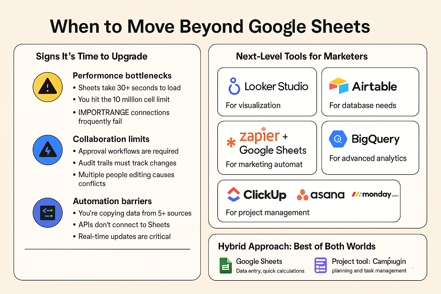
Signs It’s Time to Upgrade
Performance bottlenecks:
- Sheets take 30+ seconds to load or recalculate
- You hit the 10 million cell limit
- Collaborators report constant “Loading…” states
- IMPORTRANGE connections frequently fail
Collaboration limits:
- You need version control beyond “View history”
- Approval workflows are required before data updates
- Audit trails must track who changed what and when
- Multiple people editing causes constant conflicts
Automation barriers:
- You’re manually copying data from 5+ sources daily
- APIs don’t connect to Sheets directly
- Real-time updates are critical (Sheets has ~1 minute delay)
- Complex calculations exceed formula capabilities
Next-Level Tools for Marketers
For visualization: Looker Studio (formerly Data Studio)
- Connects directly to Google Sheets, Ads, Analytics, and 800+ data sources
- Builds interactive dashboards with drill-downs and filters
- Free for most use cases
- Best for: Client reporting, executive dashboards, real-time campaign monitoring
For database needs: Airtable
- Combines spreadsheet interface with database power
- Better at handling relational data (connecting tables)
- Robust automation and integrations
- Best for: Content calendars, project management, CRM customization
For marketing automation: Zapier + Google Sheets
- Automates data flow between 5,000+ apps
- No coding required for basic automations
- Can trigger actions when sheet data changes
- Best for: Lead routing, automated reporting, cross-platform data sync
For advanced analytics: BigQuery
- Google’s data warehouse for massive datasets
- SQL-based analysis
- Connects to Sheets for query results
- Best for: Enterprise data, complex joins, historical analysis across years
For project management: ClickUp, Asana, Monday.com
- Built-in reporting and dashboards
- Task-based workflow management
- Automated notifications and dependencies
- Best for: Team collaboration, campaign planning, resource allocation
Hybrid Approach: Best of Both Worlds
You don’t have to abandon Sheets completely. Many marketers use a hybrid setup:
- Google Sheets: Data entry, quick calculations, ad-hoc analysis
- Looker Studio: Automated visual dashboards for stakeholders
- Project tool: Campaign planning and task management
- Sheets as middleware: Query results from BigQuery, feed into Looker Studio